Chemical reactions that accompany electro-migration and electro-remediation of contaminated soils

1. Principles

An electric potential gradient in a soil lets the cations in the pore water move to the cathode and the anions to the anode, counter-balancing the negative and positive charges on the electrodes. It can be used to obtain the diffusion rate of Cl^- in concrete that is otherwise too slow to be measurable in laboratory experiments. And it can assist in the remediation of contaminated soils together with the oxidation/reduction reactions that accompany the application of an electric field. Details of the calculations can be found in Appelo, 2017, Solute transport solved with the Nernst-Planck equation for concrete pores with 'free' water and a double layer, Cem. Concr. Res. 101, 102-113.

The flux due to the gradients in concentration and electric potential is given by the Nernst-Planck equation:

(1)

where J_i is the flux of ion i (mol/m²/s), D is the diffusion coefficient (m²/s), c is the concentration (mol/m³), x is distance (m), z is the charge number, F is the Faraday constant (96485.3 C/eq), R is the gas constant (8.3145 V·C/eq/K), T is temperature (K), and V is potential (Volt).
For a concentration of zc = 1 meq/L, the flux given by a concentration gradient dc / dx = 1 mol/m⁴ is equal to the flux from a potential gradient dV / dx = 0.026 V/m. Thus, if we apply a (more realistic) potential gradient of 10's of Volts/m, diffusional transport is enhanced by orders of magnitude. There are a number of physical and chemical processes that accompany electro-migration that can be calculated with PHREEQC. First, let's look at the current that is generated since it allows to check the code's calculations easily.
Any local charge imbalance that results from the opposite transport of cations and anions is compensated by H⁺ or OH^- because they move faster, or by oxidation or reduction of water or the solutes in the cathode and anode cells, or of the electrodes. A current will be measured when the generated electrons enter the anode and flow out of the cathode. We take a sample with porosity of 0.1 filled with 0.3 M NaCl solution, diameter of 0.1 m, 30 mm long, thus 23.6 mL water. Two boundary reservoirs of 1 L also contain 0.3 M NaCl solution. Assume D = 1e-9 m²/s for all solutes, a tortuosity squared of 10, and apply 3 V / 30 mm. The flux of Na⁺ is -1.168e-4 eq/m²/s * 7.85e-4 m² = -9.175e-8 eq/s * F = -8.85 mC/s. The current is -8.85 mA due to Na⁺ transport. The total current is J(Na⁺) + -J(Cl^-) = 2 * -8.85 = -17.7 mA.

Figure 1. The (negative) current calculated by PHREEQC over time, given by the special basic term 'current_A', from the H2 generated, and from the concentration changes in the cathode cell (PHREEQC input file current1.phr). The current 'from H2 in cell 0' (green line, overlaps with current_A) is calculated from the moles of H2 that are captured in             EQUILIBRIUM_PHASES 0; H2(g) -10 0 when the concentration is higher than 10-13.2 M (SI = -10). The current 'from Na+ transport' is calculated from the concentration increase in the cathode cell (blue line). The orange line, marked with '+ Cl-' gives the sum of Na+ and Cl- transport. After 10 hours, the sum is smaller than the total current (red and green lines), because OH-, that is generated by the reduction reaction contributes significantly to the current (see figure 3 below). The magenta crosses give the sum of Na+, Cl- and OH- transport, which is the same as the actual current.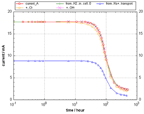

At zero time, the current agrees with what was calculated before. But as time progresses, the ions move into the boundary reservoirs, and the smaller concentrations in the pore water of the sample can only conduct a smaller current with a constant potential difference over the column.
To find the details of the current decrease over time, we must look at the Nernst-Planck equation. The electric flux of the ions is directly proportional to their concentration, and the concentration will be higher near the attracting electrode than at the other end where the ion is repelled. It means that the sample is depleted of the ion, or, in other words, that the concentration decreases in the column. Consequently, the current decreases, and it must do so equally, everywhere in a circuit that has no capacitor. But then, the potential gradient must be higher where the concentration is smaller. And this is the case indeed, as shown in Figure 2.

Figure 2. (Left) The progress of the Na⁺ concentration with time in the sample and the boundary cells where the potential is applied. The Cl^- concentration is a mirror of the Na⁺ concentration and is shown when the PHREEQC file is run. (Right) The potential over the sample at the same time-steps. Initially, the gradient is linear when the concentrations are the same everywhere. But when the concentrations change, the gradient changes as well, and it becomes highest where the concentrations are smallest, maintaining so at all points in the column the same, but smaller than initial current.

The current due to Na⁺ and Cl^-, divided by the total current, give the transport numbers of the ions (the fraction of the current transported by an ion). Clearly, it changes when the pH changes markedly in the cell. If one of the solute ions takes part in the electrode reactions, for example, Cl^- in an Ag/AgCl electrode, the pH change is insignificant, since the reactions AgCl = Ag⁺ + Cl^- and Ag⁺ + e^- = Ag are not depending on H⁺ and OH^-.

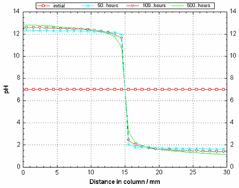
The charge balancing by OH^- and H⁺ is evident in the pH change shown in Figure 3. The concentrations of the two ions are significant, but at the opposite ends of the column, and their transport must be included in the calculations, while the activities of OH^- and H⁺ are connected by the law of mass action:

             [OH^-][H⁺] = 10^-14 (at 25°C)                                     (2).

Figure 3. The pH for a number of timesteps as a function of distance in the column. At high pH, OH- balances the surplus of positive charge at the cathode, at low pH, H+ balances the negative charge at the anode. The hydroxyls and protons are generated by reduction and oxidation of water:             H2O = OH- + ½ H2 - e-, and             H2O = 2 H+ + ½ O2 + 2 e-. Thus, at the cathode and anode, the redox potential decreases and increases, respectively. In the present calculations, it is assumed that the oxidation and reduction are sufficiently fast to calculate both as equilibrium reactions (but PHREEQC can calculate it as a kinetic reaction with the Butler-Volmer equation).

We started with equal diffusion coefficient of 1e-9 m²/s for all solute species. But if we set D(Cl^-) = 2e-9 m²/s, the initial current is 17.7 * (1 + 2) / 2 = 26.55 mA. You can check this, uncommenting the definition of the Cl-solution species in the file. And, if phreeqc.dat is used, which contains definitions of individual diffusion coefficients of the species, the initial current will be 29.7 mA.

When phreeqc.dat is used, all the solutes have their own diffusion coefficient, and the protons, generated at the anode, diffuse 7 times faster than Na⁺, and about twice faster than the hydroxyls. As a result, the pH-jump, that is in the middle of the column in figure 3, will move towards the cathode, and the concentration patterns of the ions become more asymmetric, as shown in figure 4. The increasing gradient of the pH enhances diffusional transport of OH^- from the cathode reservoir, and this flow becomes an even more important part of the current.
Thus, when the file is run with phreeqc.dat, the current initially increases with time, in contrast with the results shown in Figure 1. And the current, calculated from the transfer of Na⁺ and Cl^- in the cathode reservoir, is now much smaller than the actual current. However, when the Na⁺ and Cl^--concentrations become near-zero, the current drops like in Figure 1.

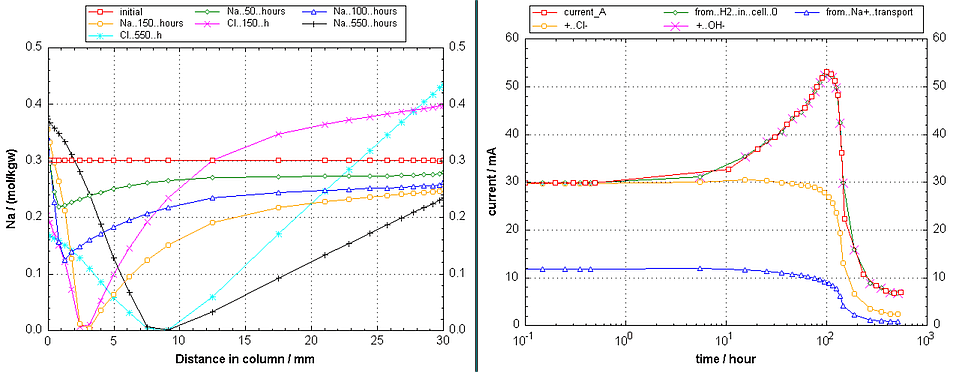
Figure 4. (Left) Time-changes of the Na⁺- and Cl^--concentrations vs. distance when phreeqc.dat is used. Note that transport of Na⁺ is slower than of Cl^- (the concentration changes of Na⁺ in the reservoirs are smaller), because the diffusion coefficient is smaller (compare with Figure 2). (Right) The current as a function of time.

For checking the code, Figure 5 compares the steady state concentrations and potential with an analytical solution (Krabbenhøft and Krabbenhøft, 2008, Cement and Concrete Research 38, 77-88), using input file current2.phr. The OH^--concentration in the two boundary solutions is 108 mmol/kgw, and H⁺ is negligible according to eqn (2). For the model calculations, a grid is defined with cell-lengths increasing log-wise from the end-cells, in total 23 cells for the 10 mm sample. It is of interest to note that in most of the column, the ratios of the concentrations are determined by the ratios in the source reservoir, thus, the anode reservoir for the cations (K⁺ / Na⁺ = 83 / 25 = 3.32), and the cathode reservoir for the anions (Cl^- / OH^- = 500 / 108). For example, at 5 mm, K⁺ / Na⁺ = 275 / 82.9 (= 3.32), and Cl^- / OH^- = 295 / 63.6.
The analytical solution is independent of the diffusion coefficients, and it does not matter whether wateq4f.dat is used as database, or phreeqc.dat (with individual diffusion coefficients for the solute species). However, with phreeqc.dat the runtime is longer because the diffusion coefficient of H⁺ is higher; the runtime can be reduced, redefining -dw 1e-9 for H⁺ since the proton concentration is everywhere negligible in this example.

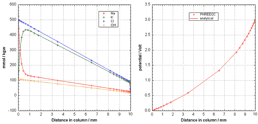
Figure 5. (Left) Steady state concentrations of Na⁺-, K⁺-, Cl^-- and OH^--concentrations with distance. (Right) The steady state potential over the sample. Lines from an analytical solution, + symbols from PHREEQC.

It is well known that the diffusion coefficients in an electric field vary with solution composition, but in the calculations for Figure 5 they are constant since the analytical solution cannot account for such variations. In PHREEQC, an option is available to let diffusion coefficients change similar to the calculation of the specific conductance of a solution (SC), see calculate the specific conductance of a solution with PHREEQC. The specific conductances calculated from the current with Ohm's law and from SC are then identical, as illustrated in Figure 6. The option is invoked when 'true' is added to the line with identifier -multi_D: -multi_d true 1e-9 1 0.0 1 true see file SC_Ohm.phr. The file defines two boundary cells, and one cell for the column with 1 m3 water and default length of 1 m, and thus with a surface area of 1 m2. The electric field is 1 V/m. The specific conductance from Ohm's law is 1 / R = I / E, where 1 / R is the specific conductance (S/m), I is the current density (Ampère/m2), and E is the electric field (1 V/m).

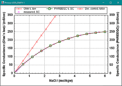Figure 6. The specific conductance calculated from the current             with Ohm's law and from SC are equal when the diffusion             coefficients are corrected for ionic strength. The red line with             the XCross symbols shows the current`s specific conductance             when the diffusion coefficients remain constant at their infinite-             dilution values. The magenta crosses show measured SC`s.

Finally, can the code calculate uphill diffusion that results from the charge imbalance due to different diffusion coefficients, as shown in the upgradient example?
We can define in keyword TRANSPORT that the current is fixed, and PHREEQC calculates transport with the Nernst-Planck equation, adapting the potentials in the cells to obtain the current. Fixing the current to a small value, say 1e-10 Ampère, is identical with zero-charge transfer and can be used to compare the two calculation types. Alternatively, the implicit algorithm can be used, setting -implicit true 5 in keyword TRANSPORT, with 'max_mixf' = D * Δt / Δx² = 5. The time steps then are more than 10 times larger, and the calculations 10 times faster.
The results of running file uphill_NP.phr are shown in Figure 7.

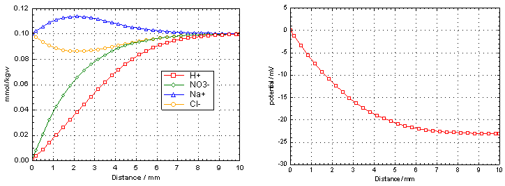
Figure 7. (Left) Concentrations of H⁺, NO₃^-, Na⁺ and Cl^- in a column showing uphill diffusion of Na⁺ and Cl^-. (Right) The potential in the column becomes negative because H⁺ diffuses faster out than NO₃^-.

Initially, the concentrations of Na⁺ and Cl^- are the same in the column and the boundary solution, while the concentrations of H⁺ and NO₃^- are higher in the column. H⁺ diffuses faster than NO₃^- from the column, and a negative potential develops that pushes Cl^- out, and attracts Na⁺ from the boundary solution. The calculated potential is as low as -23 mV after 20 minutes.
The concentration pattern shown in Figure 7 is identical with what is calculated by imposing zero-charge transfer (also shown when the file is run), although the formulas used in the calculations are different. When eqn (1) is solved with zero-charge transfer, the potential is omitted from the calculations. On the other hand, the complete calculation with the Nernst-Planck equation shows that a potential of -23 mV develops in the column that may well be measurable experimentally.

The input files current1.phr, current2.phr, SC_Ohm.phr and uphill_NP.phr use features for calculating electro-migration with PHREEQC: